The idea
Menon et al. argue a teacher's soft labels help because they approximate the Bayes posterior p(y | x), the true probability of each class given the input; the closer, the better the target. In real data nobody knows p(y | x). In this toy world it is computable exactly, so a student can be distilled from the perfect teacher. That bounds what soft labels can do for a given student size.
How it works
The world generates data in two stages: pick a class y uniformly from 20 and one of its 8 modes (sub-clusters) uniformly; draw a latent point z from a Gaussian around that mode (standard deviation 1.5 in every direction); then map it to the input with an invertible warp x = R1 · z + 0.5 · sin(R2 · z).
lik[c] = sum over modes m of exp(-|z - centre[c, m]|^2 / (2 * 1.5^2))
p(y = c | z) = lik[c] / sum_c' lik[c']- Since every class and mode is equally likely and all Gaussians share one spread, the posterior is the ratio of summed Gaussian densities above (shared constants cancel).
- The warp is a bijection (each
xcomes from exactly onez), sop(y | x) = p(y | z). - Compute the posterior for every transfer input.
- Distill the student on it with KD at
T = 1: the posterior is already the right probability and needs no softening. - The Bayes-optimal classifier picks
argmax p(y | x); its test accuracy is the ceiling no model can beat.
The code, line by line
World._posterior in lab/world.py:
diff = z[:, None, None, :] - self.centres[None]has shapeN × C × M × d(inputs, 20 classes, 8 modes, 12 dimensions): the offset from every input to every mode centre.logp = -0.5 * (diff ** 2).sum(-1) / s.noise ** 2is each mode's log-density up to a shared constant, shapeN × C × M.m = logp.max(axis=(1, 2), keepdims=True)is each input's largest log-density. Subtracting it beforenp.expkeeps the largest term atexp(0) = 1, so not every class underflows to zero; it cancels in the ratio.lik = np.exp(logp - m).sum(-1)sums over modes: the (scaled) likelihood of each class.lik / lik.sum(1, keepdims=True)normalizes over classes.
World.sample calls it on the latent z and stores the result as Split.bayes. With a non-uniform class_probs, it multiplies in the class prior and renormalizes.
run_bayes in lab/methods.py: soft = np.log(np.concatenate([d.train.bayes, d.pool.bayes]) + 1e-8) turns the posterior for all 28k transfer inputs into logits (softmax(log p) = p). FixedSource(X, None, ..., t_logits=soft) uses them as fixed targets with no labels, and KD(T=1) matches them. The comparison arms are scratch (labels only, on the 8k labeled inputs) and distill from the trained 3x256 teacher at its default T = 1, so both teachers use the same temperature. The ceiling row is (d.test.bayes.argmax(1) == d.test.y).mean().
What the simulations show
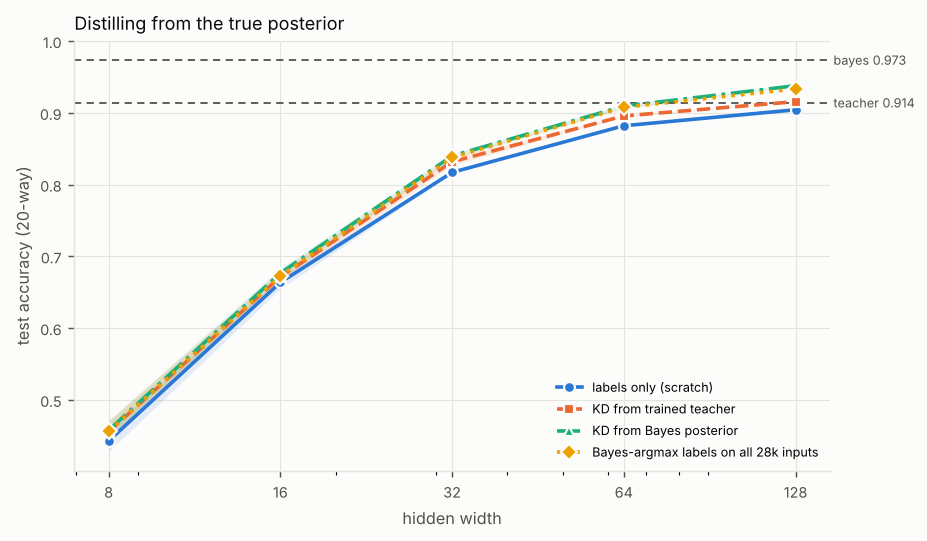
oracle_teacher (3 seeds, 3000 steps, both KD arms at T = 1, test accuracy; the Bayes ceiling is 0.9734 and the trained teacher scores 0.9139):
| student | labels only | KD from trained teacher | KD from Bayes posterior | Bayes-argmax labels on all 28k inputs |
|---|---|---|---|---|
| 2x8 | 0.4428 | 0.4556 | 0.4577 | 0.4562 |
| 2x16 | 0.6637 | 0.6714 | 0.6766 | 0.6728 |
| 2x32 | 0.8170 | 0.8318 | 0.8399 | 0.8378 |
| 2x64 | 0.8820 | 0.8957 | 0.9093 | 0.9077 |
| 2x128 | 0.9042 | 0.9156 | 0.9378 | 0.9333 |
The perfect teacher beats the trained one at every width, and the gap grows with the student: at 2x8 they are within seed noise, at 2x128 the posterior gives 0.9378 against 0.9156, more accurate than the 3x256 teacher itself. Only wide students can use a better target.
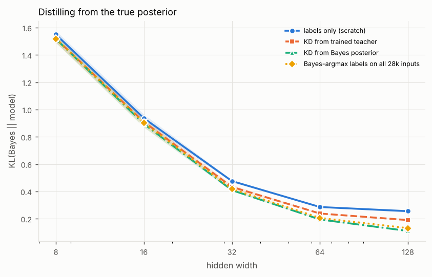
The last column trains on the posterior's top class as hard labels and recovers almost all of the gain. So most of the benefit is not the soft shape but labels on all 28k inputs: 3.5 times the 8k labeled set, each the most probable class rather than the sampled one. The soft part shows mostly in calibration: at 2x128, KL divergence to the true posterior is 0.1101 for the soft student, 0.1306 for the hard one, and 0.1900 for the student of the trained teacher.
This page's runs (1000 steps, seed 0; labels only, KD from trained teacher, KD from posterior): width 16 gave 0.5803, 0.5850, 0.5898; width 64 gave 0.8514, 0.8596, 0.8682; width 128 gave 0.9010, 0.9032, 0.9172.
When it breaks
- No real dataset has an exact posterior: this is a measuring stick, not a deployable technique.
- The formula relies on equal class and mode weights and one shared noise level; with unequal priors the weights must be multiplied in, as
sampledoes forclass_probs. - It only works because the warp is invertible. With a lossy map from
ztox,p(y | z)is notp(y | x). - Even perfect targets do not remove the capacity limit: a 2x8 student reaches 0.4577 against a 0.9734 ceiling.
Try this
- Set student width to 128. Compare the posterior row with the trained teacher's own accuracy in the teacher row, 0.9150. That is the copy the Run button loads, trained again with the same recipe; the experiment above used an earlier training, which scored 0.9139.
- Set student width to 8, then 16. See how much of the gap between labels and posterior survives when the student is tiny.
- At student width 64, the gap between "KD from trained teacher" and "KD from exact posterior" is what a better teacher could buy at this size.
Going further
Real systems approximate the posterior with better teachers: ensembles, temperature-scaled calibration, or more training data. Menon et al. frame distillation as variance reduction: soft targets close to p(y | x) give a lower-variance estimate of the risk than one-hot labels. For the cockpit's detector this says what to want in a teacher: calibrated, accurate probabilities on the student's training inputs. lab/world.py:World._posterior and lab/experiments/teacher.py:oracle_teacher are the closest analogues.
Source code
The exact code that runs, read from the repository when this page was built.
World._posterior lab/world.py:92
    def _posterior(self, z: np.ndarray, chunk: int = 2000) -> np.ndarray:
        """Exact p(y|z) for the equal-weight isotropic Gaussian mixture.
        Chunked so memory stays small (it also runs in a browser)."""
        s = self.spec
        out = []
        for i in range(0, len(z), chunk):
            diff = z[i:i + chunk, None, None, :] - self.centres[None]   # n,C,M,d
            logp = -0.5 * (diff ** 2).sum(-1) / s.noise ** 2             # n,C,M
            m = logp.max(axis=(1, 2), keepdims=True)
            lik = np.exp(logp - m).sum(-1)                               # n,C
            out.append(lik / lik.sum(1, keepdims=True))
        return np.concatenate(out)
Simulation figures
Distilling from the true posterior
If the teacher's soft labels were perfect (the exact Bayes posterior), how much better would students get? This bounds what any teacher can give.
This figure did not load: the file is missing or the connection dropped. Reload the page to try again; the experiment's full table on the Results page has the same numbers.
This figure did not load: the file is missing or the connection dropped. Reload the page to try again; the experiment's full table on the Results page has the same numbers.
Papers
- Menon et al. A Statistical Perspective on Distillation (2021)