The idea
In a residual network each layer adds to a running vector, the residual stream: h ← h + f(h). If a layer's output points almost the same way as its input, the layer barely changes the stream, and deleting it should cost little. ShortGPT measures this with block influence, BI = 1 - cos(input, output), averaged over calibration data. It deletes the layers with the lowest BI. Whole layers disappear, so the model gets proportionally faster on any hardware, with no special kernels.
How it works
- Run calibration data through the model. For each residual layer
i, record the hidden state entering it (x_i) and leaving it (x_{i+1}), one vector per token. - For each token, compute the cosine similarity
cos = x_i · x_{i+1} / (|x_i| · |x_{i+1}|). BI_i = 1 - mean(cos)over all tokens.- Sort layers by BI and delete the
klowest. Deleting a residual layer just means skipping it, since the stream passes through unchanged. - Optionally, fine-tune briefly to heal the damage.
In a transformer, a "layer" is a whole decoder block (attention plus MLP, each with its own residual add). x_i is the residual stream at the block boundary. The paper reports that on LLaMA-2 the low-BI blocks sit mostly in the later half. Removing about a quarter of them keeps most of the MMLU score, but hurts generation tasks more. Gromov et al. use a related score, the angular distance between x_i and x_{i+n}. They remove the most similar run of n consecutive blocks, then heal with QLoRA.
Why one score per layer is enough to start with: in a residual network, deleting layer i replaces x_{i+1} = x_i + f_i(x_i) with x_{i+1} = x_i. The error you introduce is exactly f_i(x_i). BI measures how much that update rotates the stream. Downstream layers see a slightly different input, but if the change is small in angle, they mostly behave the same.
The code, line by line
block_influence(net, X):
h = X, thenfor i in range(net.n_layers - 1)walks the hidden layers, skipping the output head.nxt = layer_forward(net, i, h)runs one layer. For a residual layer that ish + relu(h @ W + b), sonxtis the stream after the layer.if net.res[i]:only residual layers get a score. In the 8x128 teacher, the first hidden layer maps 12 inputs to 128, so it can't be residual. That leaves layers 1-7, and the "of 7" in the parameter label.cos = (h * nxt).sum(1) / (np.linalg.norm(h, axis=1) * np.linalg.norm(nxt, axis=1) + 1e-8)is one cosine per calibration input (each row is one example, the toy version of a token).out[i] = float(1 - cos.mean())is the BI.h = nxtmoves to the next layer, so every score is measured on the original, unpruned model. All layers are scored once, up front.
In run_block_influence, sorted(bi, key=bi.get)[:k] picks the k lowest. drop_layers deletes them. Two baselines follow: a random choice, and _greedy_drop, which tries deleting each remaining layer, keeps the one that leaves the highest accuracy on 2,000 training examples, and repeats k times.
What the simulations show
Residual 8x128 teacher, 0.9100 accuracy. Block influence by layer (512 calibration inputs):
| layer | 1 | 2 | 3 | 4 | 5 | 6 | 7 |
|---|---|---|---|---|---|---|---|
| BI | 0.0986 | 0.0790 | 0.0673 | 0.0645 | 0.0745 | 0.0808 | 0.0866 |
The middle layers change the stream least. This network has no "lazy deep layers" pattern; that is an LLM finding the toy doesn't reproduce.
| layers deleted | lowest BI | random | trial and error |
|---|---|---|---|
| 1 | 0.8560 (layer 4) | 0.8530 (layer 6) | 0.8675 |
| 2 | 0.7557 (3, 4) | 0.7632 (5, 6) | 0.8051 |
| 4 | 0.5060 (2-5) | 0.5227 (2, 4, 5, 6) | 0.5453 |
BI picks reasonable single layers. At 2 it deletes two adjacent layers and does slightly worse than random. At 4, random beats it. A greedy search that actually measures accuracy beats both.
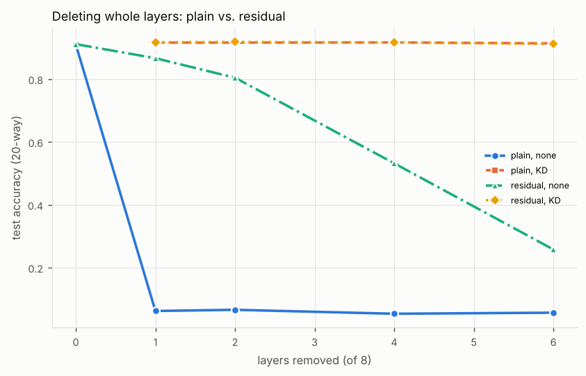
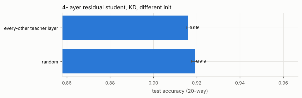
The layer_drop experiment (lab/results/layer_drop.json, recorded with an earlier training of the same teacher, which scored 0.9113) shows why residual connections matter. Deleting one layer of the plain 8x128 network drops accuracy to 0.0622, while the residual one keeps 0.8666 (greedy choice). With knowledge-distillation recovery, the residual net with 4 layers deleted returns to 0.9168 (mean of 2 seeds).
When it breaks
- Scores are computed once on the full model. After one layer is removed, the others see different inputs and their BI changes. Neighbouring low-BI layers may do overlapping work, so deleting both can hurt more than their scores suggest (see the 2-layer row).
- Cosine ignores length. A layer that grows or shrinks the stream without rotating it scores
BI ≈ 0, yet it still matters to the normalization and nonlinearities that follow. - Low BI on generic calibration text doesn't mean low importance for your task. Depth-pruned LLMs tend to keep multiple-choice benchmark scores better than open-ended generation quality.
- Plain (non-residual) networks: there is no identity path, so deleting any layer is catastrophic. BI doesn't apply.
Try this
- layers to delete (of 7) = 1: BI picks layer 4. Check whether trial and error agrees.
- Set it to 2: look for BI choosing adjacent layers 3 and 4, and the gap to trial and error.
- Set it to 4: look for random beating BI. One-shot ranking fails as more layers go.
Going further
On LLMs, follow depth pruning with a short healing fine-tune: LoRA or QLoRA on generic text, or distillation from the original model. In this repo, lab/experiments/shrink.py (the layer_drop experiment) runs the KD recovery, and lab/nn.py:MLP.drop_layer does the surgery. An iterative variant (delete one, re-score, repeat) only needs block_influence called again on the shrunken model inside a loop.
Source code
The exact code that runs, read from the repository when this page was built.
block_influence lab/layerwise.py:310
def block_influence(net: MLP, X: np.ndarray) -> dict[int, float]:
    """For every residual hidden layer i: BI = 1 - mean cos(input, output).
    A layer whose output points the same way as its input barely changes the
    residual stream, so it is the cheapest to delete."""
    out = {}
    h = X
    for i in range(net.n_layers - 1):
        nxt = layer_forward(net, i, h)
        if net.res[i]:
            cos = (h * nxt).sum(1) / (np.linalg.norm(h, axis=1) * np.linalg.norm(nxt, axis=1) + 1e-8)
            out[i] = float(1 - cos.mean())
        h = nxt
    return out
Simulation figures
Deleting whole layers: plain vs. residual
Remove k of 8 hidden layers from a deep teacher. Residual nets are said to behave like ensembles of shallow paths. Does that make depth removable? And is initializing a shallow student from the teacher's layers worth it?
This figure did not load: the file is missing or the connection dropped. Reload the page to try again; the experiment's full table on the Results page has the same numbers.
This figure did not load: the file is missing or the connection dropped. Reload the page to try again; the experiment's full table on the Results page has the same numbers.
Papers
- Men et al. ShortGPT: Layers in Large Language Models are More Redundant Than You Expect (2024)
- Gromov et al. The Unreasonable Ineffectiveness of the Deeper Layers (2024)