The idea
To get a width-16 network you can train width 16, or train something much wider, which learns faster, then prune it to width 16 and fine-tune. Li et al. (2020) argued that for large transformers under a fixed compute budget, training large and then compressing beats training small. This page tests that on MLPs, with structured (whole-neuron) pruning and self-KD: recovery by distilling from the model's own unpruned version.
How it works
- Train a
2 x startnetwork from scratch on labels. - Score its neurons with the Taylor criterion,
sum |a * dL/da|over examples (see Structured pruning). - Keep the top
targetneurons in each hidden layer. - Recover for half the original training budget, either on labels or by distilling from the unpruned
2 x startnet. - Baseline: train
2 x targetdirectly for the same total number of steps.
The code, line by line
train_big_then_compress in lab/experiments/small.py loops over target in [16, 32] and start = target * mult for mult in [1, 2, 4, 8, 16], 2 seeds each. big = scratch([start, start], s) trains the wide net for STEPS = 3,000 steps.
The mult == 1 branch is the baseline. m = scratch(big, s, steps=STEPS // 2) continues training the target-width net for the same extra 1,500 steps the pruned nets get for recovery, so every arm sees 4,500 steps in total. There is no self-KD baseline: distilling a net into an exact copy of itself has zero gradient (T * (ps - pt) / N with ps == pt).
For mult > 1, sc = neuron_importance(big, probe.X, probe.y, "taylor") scores every hidden neuron on 2,000 training examples. cut = structured_prune(big, [target, target], sc) keeps the top target per layer. That keeps only (target / start) ** 2 of the hidden-to-hidden weights. Two recoveries follow, each from a fresh cut.copy(): scratch(..., steps=STEPS // 2) on labels, and distill(cut.copy(), big, s, steps=STEPS // 2) with the wide net as teacher (KD at distill's default T=1). Both use the same learning rate as training from scratch.
run_big_then_prune in lab/methods.py is the one-seed version for this page. It runs 1,000 steps for the wide net, 500 for self-KD recovery, and 1,500 for the directly trained baseline.
What the simulations show
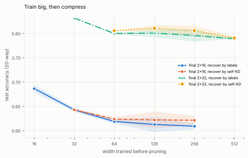
From train_big_then_compress (accuracy on 20 classes, mean of 2 seeds; every final model has the same size and the same 4,500 training steps):
| trained width | final 2x16, labels | final 2x16, self-KD | final 2x32, labels | final 2x32, self-KD |
|---|---|---|---|---|
| = target (direct) | 0.6863 | 0.8314 | ||
| 2x | 0.6425 | 0.6423 | 0.7996 | 0.8053 |
| 4x | 0.6185 | 0.6234 | 0.8004 | 0.8105 |
| 8x | 0.6124 | 0.6218 | 0.7955 | 0.8053 |
| 16x | 0.6088 | 0.6211 | 0.7886 | 0.7907 |
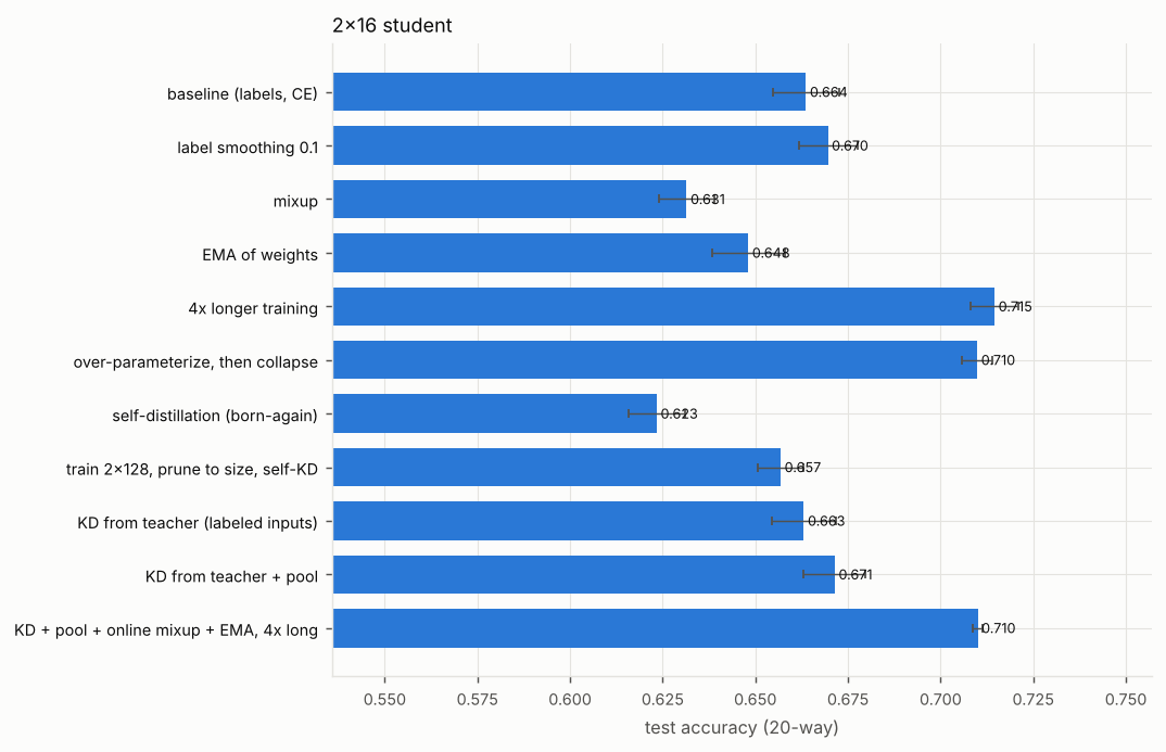
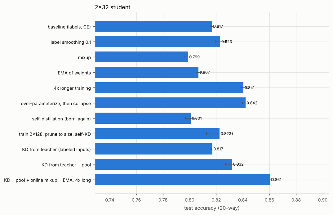
Every pruned arm is worse than training the small net directly: by at least 0.04 for 2x16 and 0.02 for 2x32. Most of the loss comes at the first doubling. Self-KD beats labels from 4x up, but never reaches the direct baseline. In small_tricks, the same recipe (2x128 → 2x16 or 2x32) with a full 3,000-step recovery landed close to plain training: 0.6568 against 0.6637 for 2x16, 0.8225 against 0.8170 for 2x32. Given enough recovery, the pruned start neither helps nor hurts much.
Page runs (1,000 + 500 steps, one seed): at the defaults (128 to 16) the 2x128 net reaches 0.9010, but pruned to 2x16 and recovered it scores 0.5037, against 0.6249 for 2x16 trained directly. Starting from 32 gives 0.5499, and from 256, 0.5024. A mild cut from 128 to 64 nearly ties: 0.8649 pruned against 0.8672 direct.
The toy does not test Li et al.'s regime: big, compute-limited models whose faster learning per step dominates, compressed lightly.
When it breaks
- Cuts too deep for recovery. Removing 7 of 8 neurons per layer leaves a damaged network that trains worse than a random init with the same budget.
- Self-KD cannot rescue a bad start. Distilling from the unpruned wide net helps a little, but a much wider teacher has functions the small net cannot represent. See the Teacher assistants page for the capacity gap.
- Unequal budgets. Here every arm gets 4,500 steps, but the wide net's steps cost far more compute. Matching FLOPs instead of steps would favour training small even more.
- In-place training.
scratchanddistilltrain their argument in place, soscratch(big, ...)in the baseline branch extendsbigitself. Copy first if you need the original.
Try this
- Keep final width 16 and step trained width through 32, 64, 128 and 256. Compare the pruned row with "trained directly" each time.
- Set final width to 64 and trained width to 128, a mild 2x cut. Compare how close the pruned net comes to the direct one with the 8x default.
Going further
Li et al.'s result rests on two facts about large transformers: bigger models reach a given loss in fewer steps, and they are more robust to quantization and pruning, so mild compression costs little. The toy reproduces neither. The YOLOv8n cockpit is train-big-then-prune by construction: it starts from a pretrained YOLOv8n and fine-tunes on only 400 bird images, so most of what the small model knows must come from the big one. Its measured cuts were mild: a ~12% channel cut recovered to 91% of native mAP@50, and a 20% cut recovered only to 0.0706 after 40 epochs. The toy's lesson is about how deep a cut goes. On the Structured pruning page, a 2x cut per layer recovered to within 0.005 of the teacher and an 8x cut never came close.
Source code
The exact code that runs, read from the repository when this page was built.
train_big_then_compress lab/experiments/small.py:76
@experiment("train_big_then_compress", G, "Train big, then compress",
            "To end up with a 2xW network, is it better to train 2xW directly or to train "
            "something much wider and prune down to 2xW? (Li et al. 2020)")
def train_big_then_compress():
    d = data()
    probe = d.train.take(2000)
    rows = []
    for target in [16, 32]:
        for mult in [1, 2, 4, 8, 16]:
            start = target * mult
            for s in SEEDS[:2]:
                big = scratch([start, start], s)
                if mult == 1:  # baseline: the same extra budget, no pruning
                    # (no self-KD arm here: distilling a net into an exact copy of
                    # itself has zero gradient)
                    m = scratch(big, s, steps=STEPS // 2)
                    rows.append(dict(target=f"final 2x{target}", start_width=start, method="labels",
                                     seed=s, **ev(m)))
                    continue
                sc = neuron_importance(big, probe.X, probe.y, "taylor")
                cut = structured_prune(big, [target, target], sc)
                rows.append(dict(target=f"final 2x{target}", start_width=start, method="labels", seed=s,
                                 **ev(scratch(cut.copy(), s, steps=STEPS // 2))))
                rows.append(dict(target=f"final 2x{target}", start_width=start, method="self-KD", seed=s,
                                 **ev(distill(cut.copy(), big, s, steps=STEPS // 2))))
    rows = agg(rows, ["target", "start_width", "method"])
    for r in rows:
        r["series"] = f"{r['target']}, recover by {r['method']}"
    return dict(rows=rows, refs=refs(), plots=[
        dict(x="start_width", y="acc", group="series", xlog=True),
    ])
Simulation figures
Train big, then compress
To end up with a 2xW network, is it better to train 2xW directly or to train something much wider and prune down to 2xW? (Li et al. 2020)
This figure did not load: the file is missing or the connection dropped. Reload the page to try again; the experiment's full table on the Results page has the same numbers.
Bag of tricks for a small model
Fixed small architecture. What actually moves its accuracy: regularizers, longer training, weight averaging, over-parameterize-then-collapse, self-distillation, a teacher, or train-big-then-shrink?
This figure did not load: the file is missing or the connection dropped. Reload the page to try again; the experiment's full table on the Results page has the same numbers.
This figure did not load: the file is missing or the connection dropped. Reload the page to try again; the experiment's full table on the Results page has the same numbers.
Papers
- Li et al. Train Large, Then Compress (2020)